Dop Properties.

Background

dopproperties started off as a project to make some of my tools more modular, flexible and maintainable. The idea was very simple: create a framework which would allow editing the DOP (dynamic operators) data tree using the SOP (surface operators) context. There were few constraints I wanted in place to shape its design and development. The framework needed to be:

• aligned with data flow model in DOPs
• data driven
• extensible
• generic
• maintainable
• modular

DOP context in Houdini is quite a different than other contexts when it comes to the flow of data. This often makes it very difficult for beginners to get a good grasp on how to efficietly and correctly setup the operators in this context.

There is another, perhaps more significant difference (more so for managers than for artists); working within this context requires a Houdini Master license or if you prefer its new name, Houdini FX license. This license is more expensive than other variants.

Most visual effects facilities try to wrap up their DOP context tools into SOP abstractions for example, a basic pyro solver or basic fluid solver abstraction within SOP context. This entails wrapping up a basic setup in DOP which would accept user inputs and create some sort of output after running a simulation (there are various motivations behind this and I will not discuss those here to keep this post as technically relevent as possible).

Unfortunately, every iteration of a SOP abstraction I have seen, is either very hacky, ugly, rigid or in most cases a combination of all these in various degrees.

dopproperties has been developed to address these requirements.

Introduction

dopproperties as the name suggests, is a framework for Houdini tool developers to author tools which are modular and allow user to drive their data tree using SOPs. dopproperties is designed to be least intrusive, is self-contained and requires a minimal amount of setup inside DOPs to work correctly.

dopproperties behaves much like data flow in DOP context where each operator really just adds, removes or modifies data to the data tree (dop objects themselves are just data).

Each dopproperties sop is designed to clearly reflect this as they have almost identical user interface to their respective DOP counterpart.

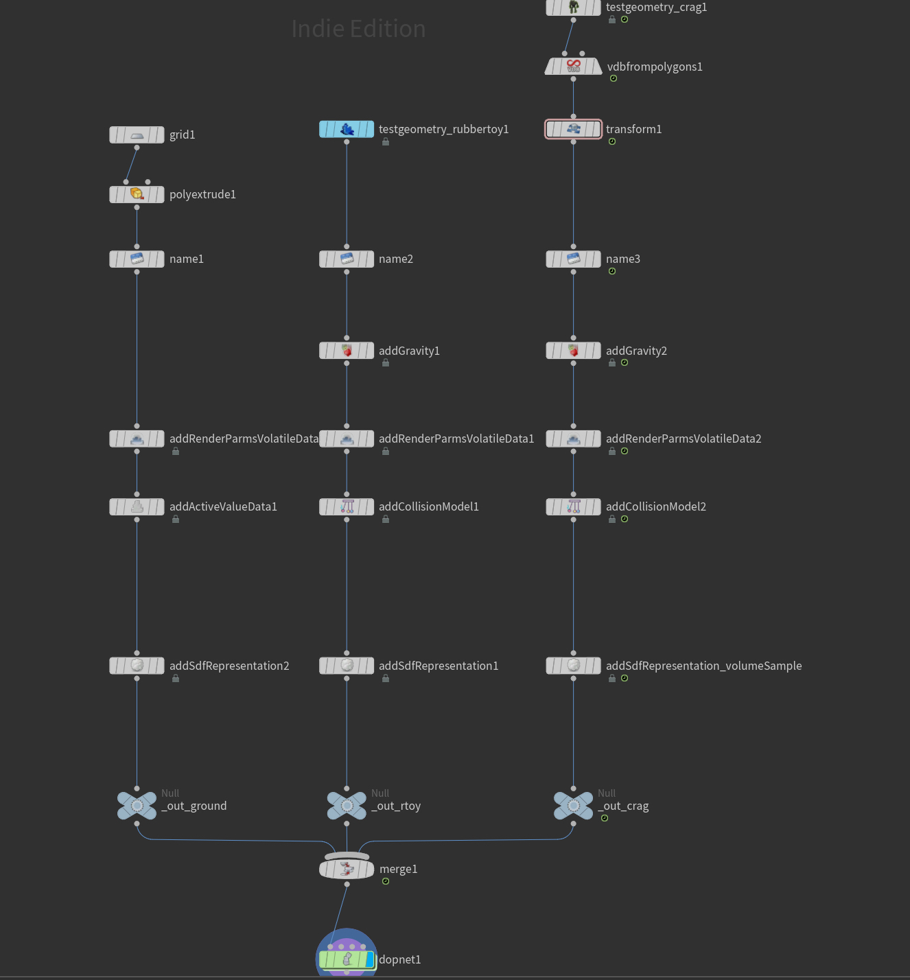
The following image shows a simple RBD simulation which has been setup using dopproperties in the SOP context. This allows users to modify, add remove objects from the simulation without ever needing to dive inside the DOP context.

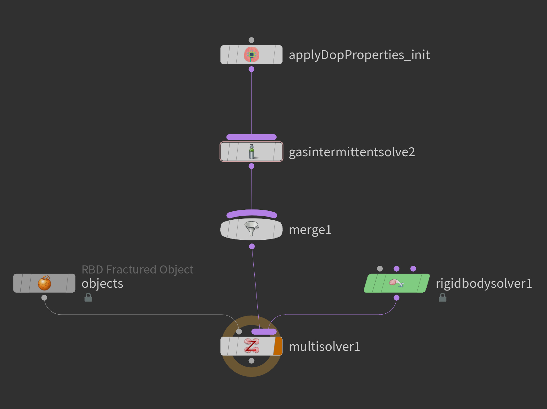
The following image shows the corressponding DOP graph which would allow dopproperties to correctly interpret and solve incoming data.

Lets have a closer look at what this SOP graph means and how it is interpreted.

1. We setup our input source geometries (grid, rubbertoy and crag) with primitive attribute “name” as is common with RBD objects.
2. Add gravity force to relevent objects.
3. Add visualisation data to the objects. By default all the objects are visible inside dop context.
4. We only need the ground to passively participate in the simulation, meaning, it should only affect other objects and not be affected by any of these obejcts. This is specified by using the Add Active Value Data sop. It tells the rigid body solver in dops to treat it as a passive object.
5. If we run the simulation now, the objects will behave in a manner rigid bodies should, however, we will notice the collisions are not accurate. This is because the objects are fairly large and there is not enough detail in their collision representations. This is remedied using the Add Sdf Representation sop and increasing the divisions (as you would have done if you were working inside dops).

All these geometry datastreams are then sent through the DOP network which in turn interprets this data and runs the simulation using one of the custom solvers Apply Dop Properties. This solver is responsible for interpreting incoming data and modifying the data tree inside dops. Since Apply Dop Properties dop is a solver, we can seamlessly combine it with all other houdini microsolvers.

Now lets have a look at the DOP graph for this simple setup.

1. We have an RBD Fractured object dop which brings in all the rbd objects using the “name” primitive attribute.
2. We run it through a multi-solver so we can have more than one solvers process the data.
3. Add in a Rigid Body Solver dop which will solve the rbds.
4. Add in Apply Dop Properties dop which interprets all the data and modifies the dop data tree. We do this before the rbd solver is run and only at the initalization stage. This is achieved using the Gas Intermittent Solver dop.

Benefits

We now have something which is similar to one of those basic rigidbody solver templates. It would seem so, however you can now completely control your dop data tree in sops. If you want to add more forces and tweak specific forces on specific objects, define new type of object, add volumetric fields to any specific objects you can! There is absolutely no need to dive inside the dop context. In fact when we look at our dop graph, there are no forces in our graph, no gravity force, no visualisaton modifiers and no Active Value dop to make any object passive! All of this is being driven by sops!

In fact if we really wanted to show off, we could define a totally custom type of dop object(akin to RBD object, Smoke object etc) in sops, on the fly using dopproperties!

If we want to update any property per frame or key-frame any property we can using the same setup with one slight modification. I will conver this example soon in another post.

This wraps up a quick intro to dopproperties and I will go over some of the more technical aspects in later posts. I am well aware, rbd solver is outdated and most of the artists favour bullet solver, however the intention here is to demonstrate the framework. We will go over few other examples in future posts.